Seasonal index standardization
James T. Thorson
Source:vignettes/web_only/seasonal_index.Rmd
seasonal_index.RmdtinyVAST can estimate seasonal spatio-temporal models
using spatially varying coefficients (Thorson et
al. 2023) to incorporate additional spatial variation by season
and then including an autoregressive spatio-temporal process across
season-within-year indices. This was originally demonstrated using
package VAST (Thorson et al. 2020), and we
here show code analyzing spring and fall bottom-trawl surveys for
yellowtail flounder in the Northwest Atlantic conducted by the NEFSC, as
well as a early-spring bottom trawl survey by DFO Canada. Here, we use a
spatio-temporal process with three seasons per year, and estimating a
lag-1 correlation (representing correlations among seasons within year)
and a lag-3 correlation (representing correlations within season among
years).
# Load data
data( atlantic_yellowtail )

# Plot data extent
ggplot( atlantic_yellowtail ) +
  geom_point( aes(x=longitude, y = latitude, col = season) ) +
  facet_wrap( vars(year) )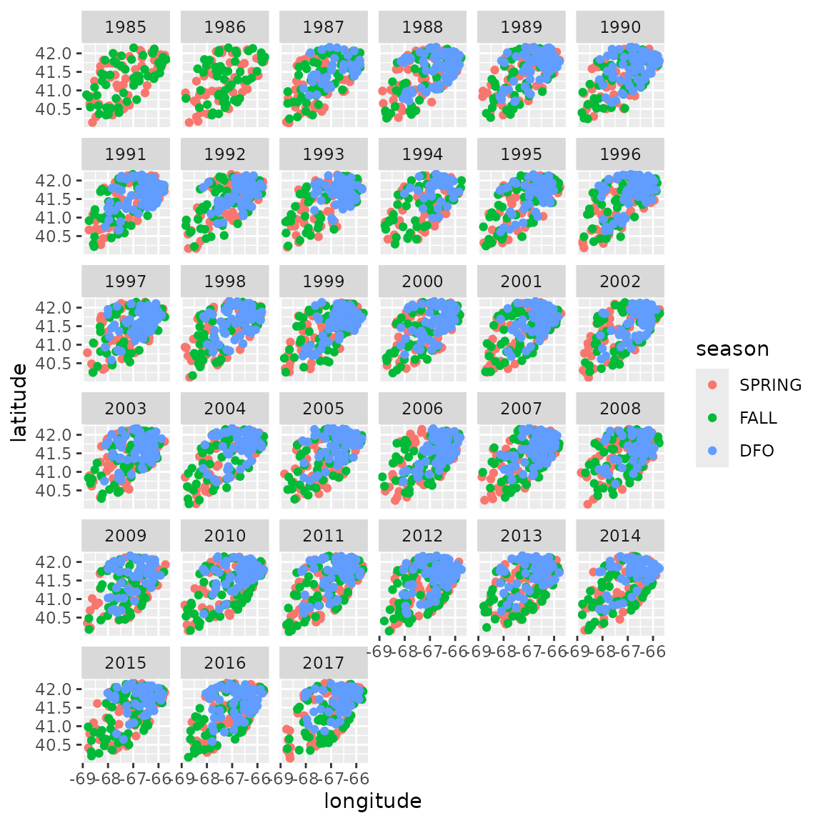
We then define a new year_season variable
# Define levels
atlantic_yellowtail$season =
  factor(atlantic_yellowtail$season, levels = c("DFO", "SPRING", "FALL"))
n_years = max(atlantic_yellowtail$year) - min(atlantic_yellowtail$year) + 1
n_seasons = nlevels(atlantic_yellowtail$season)

# convert to an integer
atlantic_yellowtail$season_year_integer =
  n_seasons * (atlantic_yellowtail$year - min(atlantic_yellowtail$year)) +
  as.numeric(atlantic_yellowtail$season) - 1

# log-scale area swept
atlantic_yellowtail$log_swept = log(atlantic_yellowtail$swept)

# Add variable column
atlantic_yellowtail$var = "density"
We then define argument spatial_varying as a formula
containing the space-season effect, and in this instance it replaces the
space_term:
# Define mesh
mesh = fm_mesh_2d(
  atlantic_yellowtail[,c('longitude','latitude')],
  cutoff = 0.2
)

# define formula log-area-swept offset, and different in mean by season
formula = weight ~ season + offset(log_swept)

# Define SVC by season
spatial_varying = ~ season

spacetime_term = "
  density -> density, 1, ar_st_season
  density -> density, 3, ar_st_year
  density <-> density, 0, sd_st
"
time_term = "
  density -> density, 1, ar_t_season
  density -> density, 3, ar_t_year
  density <-> density, 0, sd_t
"

# fit using tinyVAST
fit = tinyVAST(
  data = droplevels(atlantic_yellowtail),
  # Specification
  formula = formula,
  spatial_varying = spatial_varying,
  spacetime_term = spacetime_term,
  time_term = time_term,
  spatial_domain = mesh,
  family = tweedie("log"),
  # Indexing
  space_columns = c("longitude",'latitude'),
  time_column = "season_year_integer",
  times = seq_len(n_seasons * n_years),
  variable_column = "var",
  # Settings
  control = tinyVASTcontrol(
  #  profile = "alpha_j"
  )
)
#> Warning: The model may not have converged: non-positive-definite Hessian
#> matrix.
We can inspect output, and see that both season-within-year (lag-1) and season-across-year (lag-3) terms are significant:
summary(fit, "spacetime_term")
#>   heads      to    from parameter start lag  Estimate  Std_Error   z_value
#> 1     1 density density         1  <NA>   1 0.2460269 0.04389256  5.605207
#> 2     1 density density         2  <NA>   3 0.5267712 0.04868399 10.820213
#> 3     2 density density         3  <NA>   0 1.3015125 0.05159715 25.224503
#>         p_value
#> 1  2.080067e-08
#> 2  2.761334e-27
#> 3 2.157556e-140
We can then visualize density in selected years. To do this, we first define a predictive grid
# get sf for sampling points
sf_locs = st_as_sf(
  atlantic_yellowtail,
  coords = c("longitude","latitude")
)
sf_locs = st_sf(
  sf_locs,
  crs = st_crs("EPSG:4326")
)

# make convex hull for domain
sf_domain = st_convex_hull(
  st_union(sf_locs)
)

# Make grid in domain
sf_grid = st_make_grid(
  sf_domain,
  cellsize = c(0.1,0.1)
)
sf_grid = st_intersection(
  sf_grid, sf_domain
)

# Data frame for prediction
grid_coords = st_coordinates(st_centroid(sf_grid))
grid_coords = cbind(
  sf_grid,
  setNames( data.frame(grid_coords), c("longitude","latitude")),
  swept = as.numeric(st_area(sf_grid)) / 1e6,
  grid = seq_len(length(sf_grid))
)
We then select a set of years and seasons, predict those values, and then plot them
# season_year
newdata = expand.grid(
  season = levels(atlantic_yellowtail$season),
  year = 2013:2017,
  grid = seq_len(length(sf_grid))
)

#
newdata = merge( newdata, grid_coords )
newdata$log_swept = log(newdata$swept)

# Define levels
newdata$season =
  factor(newdata$season, levels = c("DFO", "SPRING", "FALL"))

# convert to an integer
newdata$season_year_integer =
  n_seasons * (newdata$year - min(atlantic_yellowtail$year)) +
  as.numeric(newdata$season) - 1

# Predict
newdata$logdens = predict(
  fit,
  newdata = newdata,
  what = "p_g"
)

# Censor low densities to show high densities better
newdata$logdens = ifelse(
  newdata$logdens < (max(newdata$logdens) - log(1000) ),
  NA,
  newdata$logdens
)

ggplot(newdata) +
  geom_sf( aes(fill = logdens, geometry = geometry), col = NA ) +
  facet_grid( rows = vars(year), cols = vars(season) )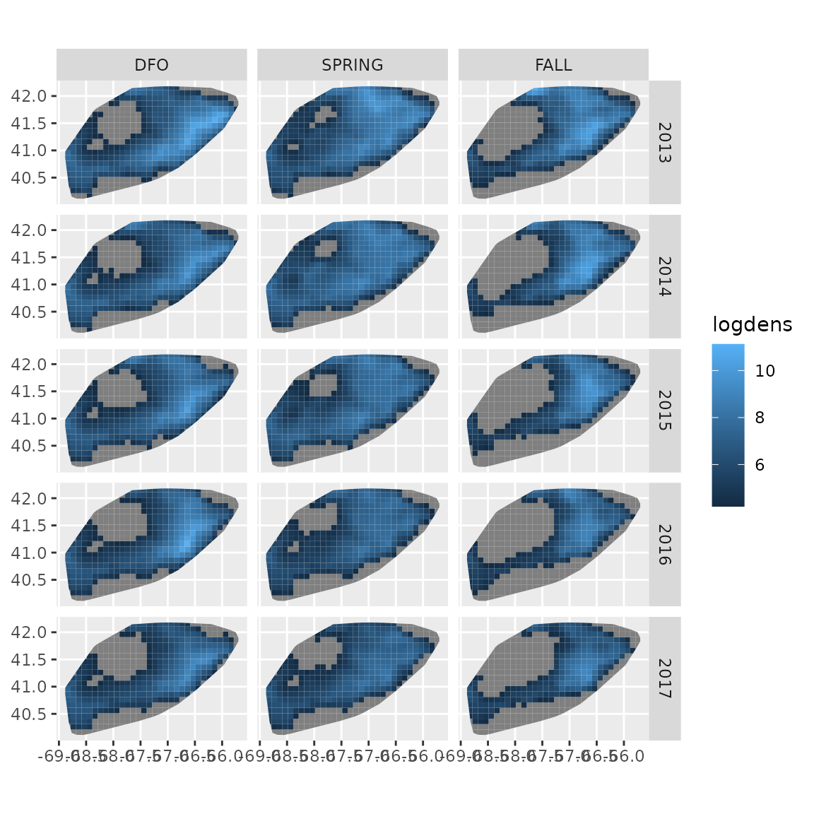
We can also project the model. To do so, we first rebuild the
newdata argument for the projection period (which would
involve forecasted covariates if we were including any) while selecting
the forecast interval:
# season_year
projdata = expand.grid(
  season = levels(atlantic_yellowtail$season),
  year = 2018:2022,
  grid = seq_len(length(sf_grid))
)

#
projdata = merge( projdata, grid_coords )
projdata$log_swept = log( projdata$swept )

# Define levels
projdata$season =
  factor(projdata$season, levels = c("DFO", "SPRING", "FALL"))

# convert to an integer
projdata$season_year_integer =
  n_seasons * (projdata$year - min(atlantic_yellowtail$year)) +
  as.numeric(projdata$season) - 1
we then use the project function, and show a
deterministic projection:
#
projdata$logdens = project(
  object = fit,
  extra_times = (n_seasons * n_years) + 1:24,
  newdata = projdata,
  what = "p_g",
  future_var = FALSE,
  past_var = FALSE,
  parm_var = FALSE
)

# Censor low densities to show high densities better
projdata$logdens = ifelse(
  projdata$logdens < (max(projdata$logdens) - log(1000) ),
  NA,
  projdata$logdens
)

ggplot(projdata) +
  geom_sf( aes(fill = logdens, geometry = geometry), col = NA ) +
  facet_grid( rows = vars(year), cols = vars(season) )
We then show a single draw from the stochastic projection
# Set seed for reproducibility
set.seed(123)

#
projdata$logdens = project(
  object = fit,
  extra_times = (n_seasons * n_years) + 1:24,
  newdata = projdata,
  what = "p_g",
  future_var = TRUE,
  past_var = FALSE,
  parm_var = FALSE
)

# Censor low densities to show high densities better
projdata$logdens = ifelse(
  projdata$logdens < (max(projdata$logdens) - log(1000) ),
  NA,
  projdata$logdens
)

ggplot(projdata) +
  geom_sf( aes(fill = logdens, geometry = geometry), col = NA ) +
  facet_grid( rows = vars(year), cols = vars(season) )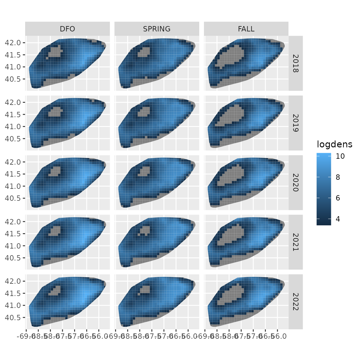
Runtime for this vignette: 7.78 mins