Vector autoregressive spatio-temporal models

James T. Thorson

library(tinyVAST)
library(fmesher)
set.seed(101)
options("tinyVAST.verbose" = FALSE)

tinyVAST is an R package for fitting vector autoregressive spatio-temporal (VAST) models. We here explore the capacity to specify the vector-autoregressive spatio-temporal component.

Univariate spatio-temporal autoregressive model

We first explore the ability to specify a first-order autoregressive spatio-temporal process, i.e., a spatial Gompertz model (Thorson et al. 2014).

Simulate univariate autoregressive process

To do so, we simulate the process:

# Simulate settings
theta_xy = 0.4
n_x = n_y = 10
n_t = 15
rho = 0.8
spacetime_sd = 0.5
space_sd = 0.5
gamma = 0

# Simulate GMRFs
R_s = exp(-theta_xy * abs(outer(1:n_x, 1:n_y, FUN="-")) )
R_ss = kronecker(R_s, R_s)
Vspacetime_ss = spacetime_sd^2 * R_ss 
Vspace_ss = space_sd^2 * R_ss

# make spacetime AR1 over time
eps_ts = mvtnorm::rmvnorm( n_t, sigma=Vspacetime_ss )
for( t in seq_len(n_t) ){
  if(t>1) eps_ts[t,] = rho*eps_ts[t-1,] + eps_ts[t,]/(1 + rho^2)
}

# make space term
omega_s = mvtnorm::rmvnorm( 1, sigma=Vspace_ss )[1,]

# linear predictor
p_ts = gamma + outer( rep(1,n_t),omega_s ) + eps_ts

# Shape into longform data-frame and add error
Data = data.frame( expand.grid(time=1:n_t, x=1:n_x, y=1:n_y), 
                   var = "logn", 
                   mu = exp(as.vector(p_ts)) )
Data$n = tweedie::rtweedie( n=nrow(Data), mu=Data$mu, phi=0.5, power=1.5 )
mean(Data$n==0)
#> [1] 0.072

Fit univariate spatio-temporal model

We then specify and fit the same model

# make mesh
mesh = fm_mesh_2d( Data[,c('x','y')] )

# Spatial variable
space_term = "
  logn <-> logn, sd_space
"

# AR1 spatio-temporal variable
spacetime_term = "
  logn -> logn, 1, rho
  logn <-> logn, 0, sd_spacetime
"

# fit model
mytinyVAST = tinyVAST( 
  space_term = space_term,
  spacetime_term = spacetime_term,
  data = Data,
  formula = n ~ 1,
  spatial_domain = mesh,
  family = tweedie() 
)
mytinyVAST
#> Call: 
#> tinyVAST(formula = n ~ 1, data = Data, space_term = space_term, 
#>     spacetime_term = spacetime_term, family = tweedie(), spatial_domain = mesh)
#> 
#> Run time: 
#> Time difference of 8.793781 secs
#> 
#> Family: 
#> $obs
#> 
#> Family: tweedie 
#> Link function: log 
#> 
#> 
#> 
#> 
#> sdreport(.) result
#>              Estimate Std. Error
#> alpha_j   -0.51039962 0.20682402
#> beta_z     0.84975932 0.07526407
#> beta_z    -0.25841509 0.03730060
#> theta_z    0.44410026 0.06898305
#> log_sigma -0.64811725 0.05006776
#> log_sigma  0.01446391 0.06494065
#> log_kappa -0.15609782 0.16446773
#> Maximum gradient component: 0.00235749 
#> 
#> Proportion conditional deviance explained: 
#> [1] 0.4812353
#> 
#> space_term: 
#>   heads   to from parameter start  Estimate  Std_Error  z_value      p_value
#> 1     2 logn logn         1  <NA> 0.4441003 0.06898305 6.437817 1.212041e-10
#> 
#> spacetime_term: 
#>   heads   to from parameter start lag   Estimate  Std_Error   z_value
#> 1     1 logn logn         1  <NA>   1  0.8497593 0.07526407 11.290372
#> 2     2 logn logn         2  <NA>   0 -0.2584151 0.03730060 -6.927908
#>        p_value
#> 1 1.464154e-29
#> 2 4.271107e-12
#> 
#> Fixed terms: 
#>               Estimate Std_Error   z_value    p_value
#> (Intercept) -0.5103996  0.206824 -2.467797 0.01359475
#> 
#> Sanity check: 
#> 
#> **Possible issues detected! Check output of sanity().**

The estimated values for beta_z then correspond to the simulated value for rho and spatial_sd.

We can compare the true densities:

library(sf)
data_wide = reshape( Data[,c('x','y','time','mu')],
                     direction = "wide", idvar = c('x','y'), timevar = "time")
sf_data = st_as_sf( data_wide, coords=c("x","y"))
sf_grid = sf::st_make_grid( sf_data )
sf_plot = st_sf(sf_grid, st_drop_geometry(sf_data) )
plot(sf_plot, max.plot=n_t )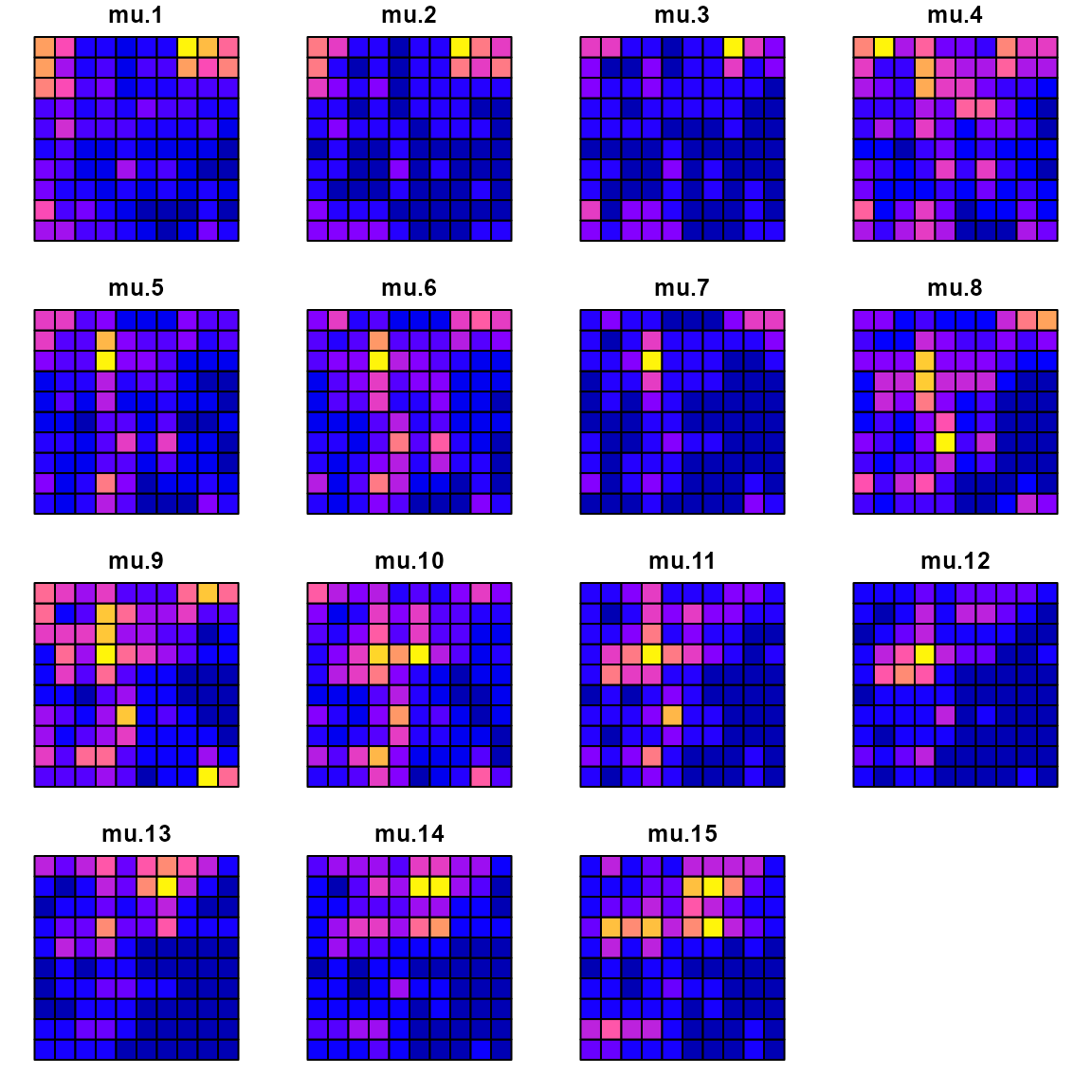

with the estimated densities:

Data$mu_hat = predict(mytinyVAST)
data_wide = reshape( Data[,c('x','y','time','mu_hat')],
                     direction = "wide", idvar = c('x','y'), timevar = "time")
sf_data = st_as_sf( data_wide, coords=c("x","y"))
sf_plot = st_sf(sf_grid, st_drop_geometry(sf_data) )
plot(sf_plot, max.plot=n_t )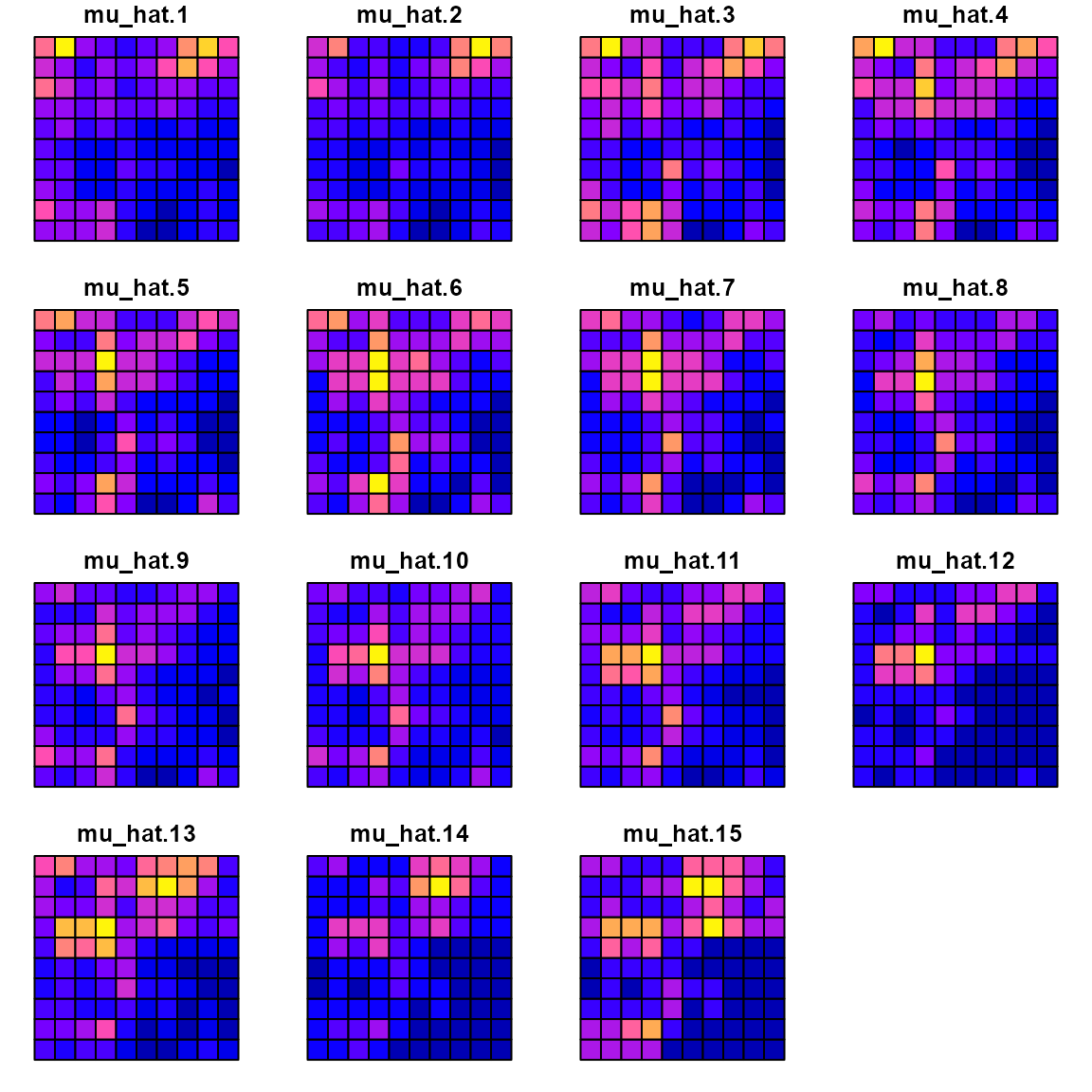

where a scatterplot shows that they are highly correlated:

plot( x=Data$mu, y=Data$mu_hat )

We can also use the DHARMa package to visualize simulation residuals:

# simulate new data conditional on fixed effects
# and sampling random effects from their predictive distribution
y_ir = simulate(mytinyVAST, nsim=100, type="mle-mvn")

#
res = DHARMa::createDHARMa( simulatedResponse = y_ir, 
                            observedResponse = Data$n, 
                            fittedPredictedResponse = fitted(mytinyVAST) )
plot(res)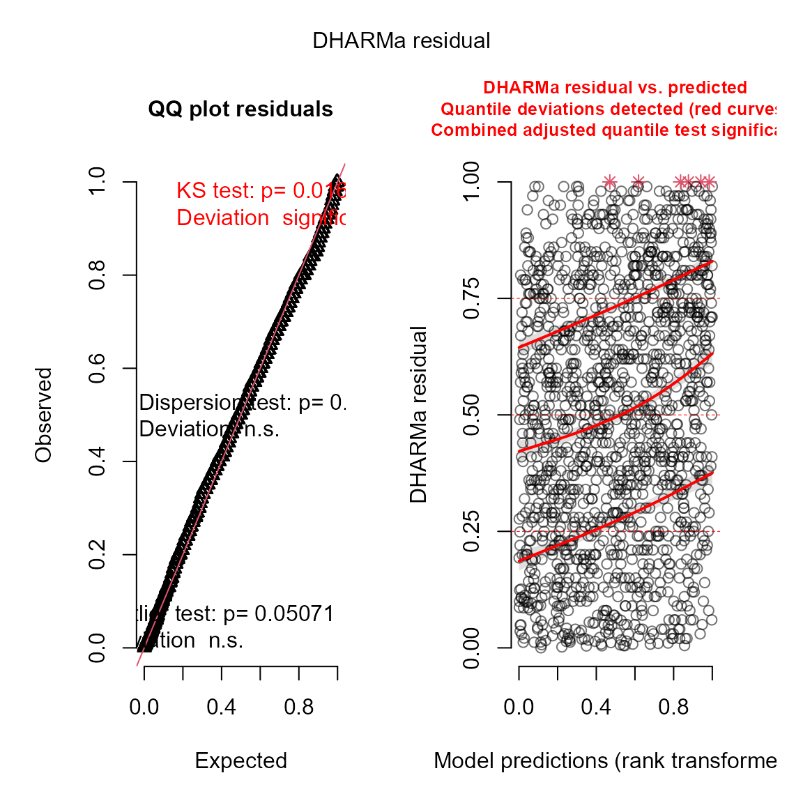

We can then calculate the area-weighted total abundance and compare it with its true value:

# Predicted sample-weighted total
(Est = sapply( seq_len(n_t),
   FUN=\(t) integrate_output(mytinyVAST, newdata=subset(Data,time==t)) ))
#>                          [,1]      [,2]      [,3]      [,4]     [,5]      [,6]
#> Estimate            69.774447 68.167140 68.249630 64.038614 58.73677 60.506551
#> Std. Error           4.733492  4.404923  4.324752  4.092695  3.88048  3.887898
#> Est. (bias.correct) 72.867385 71.288095 71.442818 67.062659 61.53693 63.391164
#> Std. (bias.correct)        NA        NA        NA        NA       NA        NA
#>                          [,7]      [,8]      [,9]     [,10]     [,11]     [,12]
#> Estimate            54.977472 58.463750 64.523936 74.895753 84.490828 76.981717
#> Std. Error           3.772124  3.863061  4.166782  4.702733  5.335558  5.141674
#> Est. (bias.correct) 57.610590 61.214901 67.544370 78.337004 88.253708 80.405033
#> Std. (bias.correct)        NA        NA        NA        NA        NA        NA
#>                         [,13]      [,14]     [,15]
#> Estimate            87.189069  96.106447 93.626602
#> Std. Error           5.514166   6.001112  6.338957
#> Est. (bias.correct) 91.106034 100.570723 98.734193
#> Std. (bias.correct)        NA         NA        NA

# True (latent) sample-weighted total
(True = tapply( Data$mu, INDEX=Data$time, FUN=sum ))
#>         1         2         3         4         5         6         7         8 
#>  70.98033  70.14925  68.40932  68.70763  58.38332  65.95801  60.52297  55.14115 
#>         9        10        11        12        13        14        15 
#>  60.02083  74.91768  86.40811  77.73359  85.88998  98.33442 105.16020

#
Index = data.frame( time=seq_len(n_t), t(Est), True )
Index$low = Index[,'Est...bias.correct.'] - 1.96*Index[,'Std..Error']
Index$high = Index[,'Est...bias.correct.'] + 1.96*Index[,'Std..Error']

#
library(ggplot2)
ggplot(Index, aes(time, Estimate)) +
  geom_ribbon(aes(ymin = low,
                  ymax = high),    # shadowing cnf intervals
              fill = "lightgrey") +
  geom_line( color = "black",
            linewidth = 1) +
  geom_point( aes(time, True), color = "red" )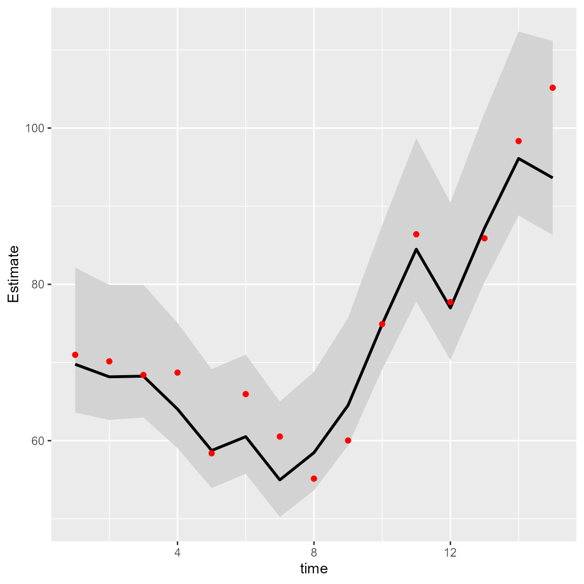

Comparison with VAST or sdmTMB

Next, we compare this against the current version of VAST (Thorson and Barnett 2017)

settings = make_settings( 
  purpose="index3",
  n_x = n_x*n_y,
  Region = "Other",
  bias.correct = FALSE,
  use_anisotropy = FALSE 
)
settings$FieldConfig['Epsilon','Component_1'] = 0
settings$FieldConfig['Omega','Component_1'] = 0
settings$RhoConfig['Epsilon2'] = 4
settings$RhoConfig[c('Beta1','Beta2')] = 3
settings$ObsModel = c(10,2)

# Run VAST
myVAST = fit_model( 
  settings=settings,
  Lat_i = Data$y,
  Lon_i = Data$x,
  t_i = Data$time,
  b_i = as.numeric(Data$n),
  a_i = rep(1,nrow(Data)),
  observations_LL = cbind(Lat=Data[,'y'],Lon=Data[,'x']),
  grid_dim_km = c(100,100),
  newtonsteps = 0,
  loopnum = 1,
  control = list(eval.max = 10000, iter.max = 10000, trace = 0) 
)

myVAST

Or with sdmTMB (Anderson et al., n.d.)

library(sdmTMB)
sdmTMB_mesh = make_mesh(Data, c("x","y"), n_knots=n_x*n_y )

start_time2 = Sys.time()
mysdmTMB = sdmTMB(
  formula = n ~ 1,
  data = Data,
  mesh = sdmTMB_mesh,
  spatial = "on",
  spatiotemporal = "ar1",
  time = "time",
  family = tweedie()
)
sdmTMBtime = Sys.time() - start_time2

The models all have similar runtimes

Times = data.frame( 
  tinyVAST = mytinyVAST$run_time,
  VAST = myVAST$total_time,
  sdmTMB = sdmTMBtime 
)
knitr::kable( cbind("run times (sec.)"=Times), digits=1)

run times (sec.).tinyVAST	run times (sec.).VAST	run times (sec.).sdmTMB
8.8 secs	NA	10.9 secs

Delta models

We can also fit this univariate spatio-temporal process using a Poisson-linked gamma delta model (Thorson 2018)

# fit model
mydelta2 = tinyVAST( 
  data = Data,
  formula = n ~ 1,
  delta_options = list(
    formula = ~ 0 + factor(time),
    spacetime_term = "logn -> logn, 1, rho"),
  family = delta_lognormal(type="poisson-link"),
  spatial_domain = mesh 
)

mydelta2
#> Call: 
#> tinyVAST(formula = n ~ 1, data = Data, family = delta_lognormal(type = "poisson-link"), 
#>     delta_options = list(formula = ~0 + factor(time), spacetime_term = "logn -> logn, 1, rho"), 
#>     spatial_domain = mesh)
#> 
#> Run time: 
#> Time difference of 8.238648 secs
#> 
#> Family: 
#> $obs
#> 
#> Family: binomial lognormal 
#> Link function: log log 
#> 
#> 
#> 
#> 
#> sdreport(.) result
#>             Estimate Std. Error
#> alpha_j    0.9673982 0.03523113
#> alpha2_j  -1.2465531 0.14981116
#> alpha2_j  -1.2927804 0.17500264
#> alpha2_j  -1.3056616 0.19172295
#> alpha2_j  -1.3218115 0.20304344
#> alpha2_j  -1.5709922 0.21258960
#> alpha2_j  -1.4450793 0.21945079
#> alpha2_j  -1.7167974 0.22626434
#> alpha2_j  -1.5448634 0.23247502
#> alpha2_j  -1.3990617 0.23308060
#> alpha2_j  -1.1251748 0.23638081
#> alpha2_j  -1.2235461 0.23877445
#> alpha2_j  -1.5131381 0.24006161
#> alpha2_j  -1.2469233 0.24216447
#> alpha2_j  -1.1278738 0.24209141
#> alpha2_j  -1.0707282 0.24334575
#> beta2_z    0.8967400 0.03512556
#> beta2_z    0.3133328 0.03906544
#> log_sigma  0.0296271 0.02475190
#> log_kappa  0.1085638 0.14818576
#> Maximum gradient component: 0.001977891 
#> 
#> Proportion conditional deviance explained: 
#> [1] 0.3295031
#> 
#> Fixed terms: 
#>              Estimate  Std_Error  z_value       p_value
#> (Intercept) 0.9673982 0.03523113 27.45862 5.482304e-166
#> 
#> Sanity check: 
#> 
#> **Possible issues detected! Check output of sanity().**

And we can again use the DHARMa package (Hartig 2017) to visualize conditional simulation quantile (a.k.a. Dunn-Smythe) residuals (Dunn and Smyth 1996):

# simulate new data conditional on fixed effects
# and sampling random effects from their predictive distribution
y_ir = simulate(mydelta2, nsim=100, type="mle-mvn")

# Visualize using DHARMa
res = DHARMa::createDHARMa( simulatedResponse = y_ir, 
                            observedResponse = Data$n, 
                            fittedPredictedResponse = fitted(mydelta2) )
plot(res)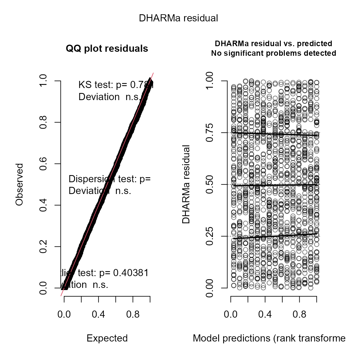

We can then use marginal and conditional AIC to compare the fit of the delta-model and Tweedie distribution:

# AIC table
AIC_table = cbind(
  mAIC = c( "Tweedie" = AIC(mytinyVAST), 
            "delta-lognormal" = AIC(mydelta2) ), 
  cAIC = c( "Tweedie" = tinyVAST::cAIC(mytinyVAST), 
            "delta-lognormal" = tinyVAST::cAIC(mydelta2) ) 
)

# Print table
knitr::kable( 
  AIC_table,
  digits=3
)

	mAIC	cAIC
Tweedie	2501.480	2356.787
delta-lognormal	2947.194	2848.163

Bivariate vector autoregressive spatio-temporal model

We next highlight how to specify a bivariate spatio-temporal model with a cross-laggged (vector autoregressive) interaction Thorson et al. (2019). ## Simulate bivariate model

We first simulate artificial data for the sake of demonstration:

# Simulate settings
theta_xy = 0.2
n_x = n_y = 10
n_t = 20
B = rbind( c( 0.5, -0.25),
           c(-0.1,  0.50) )

# Simulate GMRFs
R = exp(-theta_xy * abs(outer(1:n_x, 1:n_y, FUN="-")) )
d1 = mvtnorm::rmvnorm(n_t, sigma=0.2*kronecker(R,R) )
d2 = mvtnorm::rmvnorm(n_t, sigma=0.2*kronecker(R,R) )
d = abind::abind( d1, d2, along=3 )

# Project through time and add mean
for( t in seq_len(n_t) ){
  if(t>1) d[t,,] = t(B%*%t(d[t-1,,])) + d[t,,]
}

# Shape into longform data-frame and add error
Data = data.frame( expand.grid(time=1:n_t, x=1:n_x, y=1:n_y, "var"=c("d1","d2")),
                   mu = exp(as.vector(d)))
Data$n = tweedie::rtweedie( n=nrow(Data), mu=Data$mu, phi=0.5, power=1.5 )

Fit bivariate model

We next set up inputs and run the model:

# make mesh
mesh = fm_mesh_2d( Data[,c('x','y')] )

# Define DSEM
dsem = "
  d1 -> d1, 1, b11
  d2 -> d2, 1, b22
  d2 -> d1, 1, b21
  d1 -> d2, 1, b12
  d1 <-> d1, 0, var1
  d2 <-> d2, 0, var1
"

# fit model
out = tinyVAST( spacetime_term = dsem,
           data = Data,
           formula = n ~ 0 + var,
           spatial_domain = mesh,
           family = tweedie() )
#> Warning: The model may not have converged. Maximum final gradient:
#> 0.0108368453778236.
out
#> Call: 
#> tinyVAST(formula = n ~ 0 + var, data = Data, spacetime_term = dsem, 
#>     family = tweedie(), spatial_domain = mesh)
#> 
#> Run time: 
#> Time difference of 29.48807 secs
#> 
#> Family: 
#> $obs
#> 
#> Family: tweedie 
#> Link function: log 
#> 
#> 
#> 
#> 
#> sdreport(.) result
#>               Estimate Std. Error
#> alpha_j    0.090202981 0.11486664
#> alpha_j   -0.099500541 0.10318987
#> beta_z     0.553897565 0.07628808
#> beta_z     0.536424139 0.07383380
#> beta_z    -0.225705467 0.07606824
#> beta_z    -0.070945613 0.06259109
#> beta_z     0.336688292 0.01863795
#> log_sigma -0.696754581 0.02881155
#> log_sigma -0.005321748 0.05462454
#> log_kappa -0.635425879 0.10547175
#> Maximum gradient component: 0.01083685 
#> 
#> Proportion conditional deviance explained: 
#> [1] 0.4057952
#> 
#> spacetime_term: 
#>   heads to from parameter start lag    Estimate  Std_Error   z_value
#> 1     1 d1   d1         1  <NA>   1  0.55389757 0.07628808  7.260604
#> 2     1 d2   d2         2  <NA>   1  0.53642414 0.07383380  7.265293
#> 3     1 d1   d2         3  <NA>   1 -0.22570547 0.07606824 -2.967144
#> 4     1 d2   d1         4  <NA>   1 -0.07094561 0.06259109 -1.133478
#> 5     2 d1   d1         5  <NA>   0  0.33668829 0.01863795 18.064666
#> 6     2 d2   d2         5  <NA>   0  0.33668829 0.01863795 18.064666
#>        p_value
#> 1 3.853647e-13
#> 2 3.722318e-13
#> 3 3.005797e-03
#> 4 2.570136e-01
#> 5 6.048658e-73
#> 6 6.048658e-73
#> 
#> Fixed terms: 
#>          Estimate Std_Error    z_value   p_value
#> vard1  0.09020298 0.1148666  0.7852844 0.4322868
#> vard2 -0.09950054 0.1031899 -0.9642471 0.3349220
#> 
#> Sanity check: 
#> 
#> **Possible issues detected! Check output of sanity().**

The values for beta_z again correspond to the specified value for interaction-matrix B

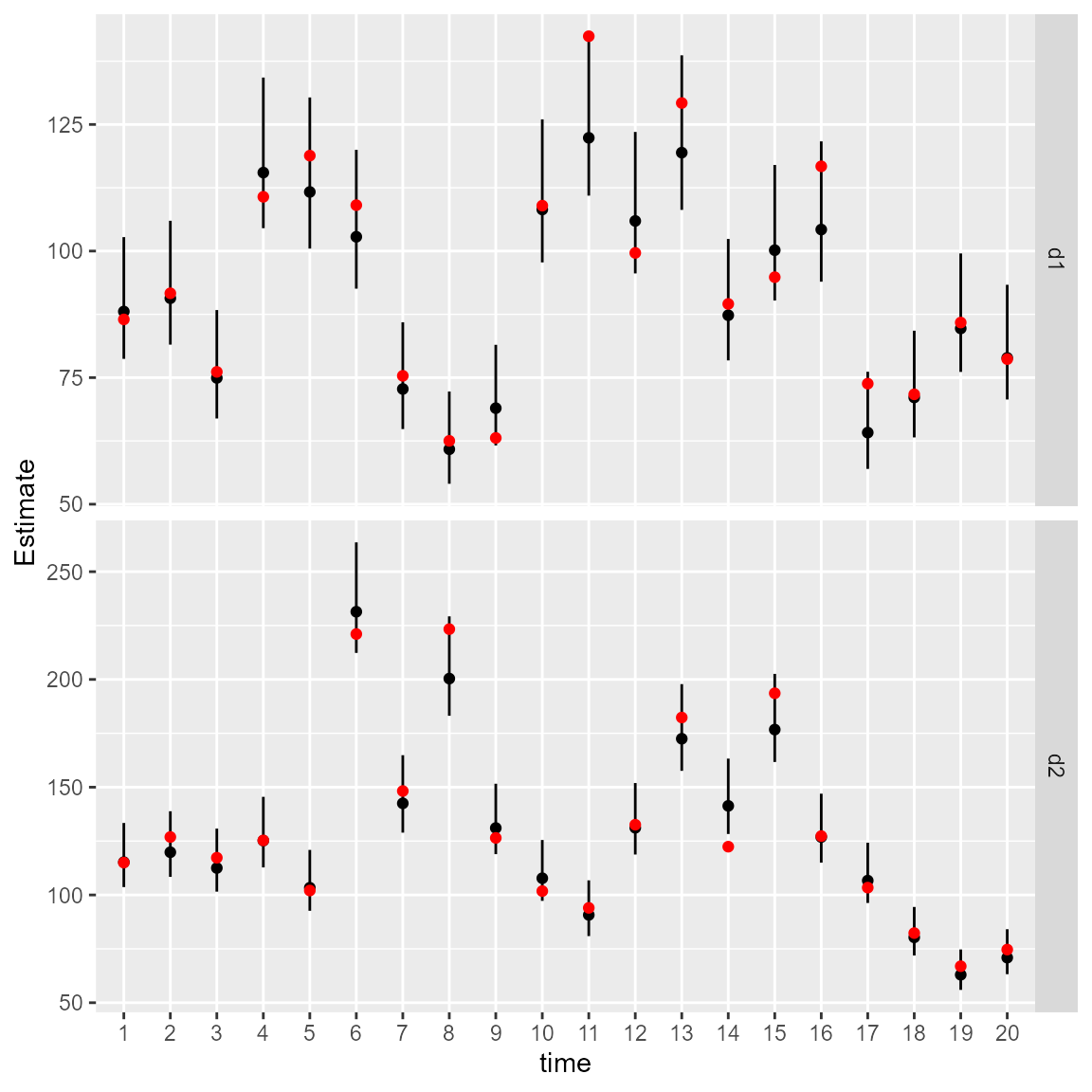
We can again calculate the area-weighted total abundance and compare it with its true value:

# Predicted sample-weighted total 
# for each year-variable combination
Est1 = Est2 = NULL
for( t in seq_len(n_t) ){
  Est1 = rbind(Est1, integrate_output( 
    out, 
    newdata = subset(Data, time==t & var=="d1")
  ))
  Est2 = rbind(Est2, integrate_output( 
    out, 
    newdata = subset(Data, time==t & var=="d2")
  ))
}

# True (latent) sample-weighted total
True = tapply( 
  Data$mu, 
  INDEX=list("time"=Data$time,"var"=Data$var), 
  FUN=sum 
)

# Make long-form data frame for ggplot
Index = data.frame( 
  expand.grid(dimnames(True)), 
  True = as.vector(True),
  rbind(Est1, Est2)
)

# Format intervals for ggplot
Index$low = Index[,'Est...bias.correct.'] - 1.96*Index[,'Std..Error']
Index$high = Index[,'Est...bias.correct.'] + 1.96*Index[,'Std..Error']

#
library(ggplot2)
ggplot(Index, aes( time, Estimate )) +
  facet_grid( rows=vars(var), scales="free" ) +
  geom_segment(aes(y = low,
                  yend = high,
                  x = time,
                  xend = time) ) +
  geom_point( aes(x=time, y=Estimate), color = "black") +
  geom_point( aes(x=time, y=True), color = "red" )

Works cited

Anderson, Sean C., Eric J. Ward, Philina A. English, Lewis A. K. Barnett, and James T. Thorson. n.d. “sdmTMB: An R Package for Fast, Flexible, and User-Friendly Generalized Linear Mixed Effects Models with Spatial and Spatiotemporal Random Fields.” Journal of Open Source Software, 2022.03.24.485545. https://doi.org/10.1101/2022.03.24.485545.

Dunn, Peter K., and Gordon K. Smyth. 1996. “Randomized Quantile Residuals.” Journal of Computational and Graphical Statistics 5 (3): 236–44. http://www.tandfonline.com/doi/abs/10.1080/10618600.1996.10474708.

Hartig, Florian. 2017. “DHARMa: Residual Diagnostics for Hierarchical (Multi-Level/Mixed) Regression Models.” R Package Version 0.1 5.

Thorson, James T. 2018. “Three Problems with the Conventional Delta-Model for Biomass Sampling Data, and a Computationally Efficient Alternative.” Canadian Journal of Fisheries and Aquatic Sciences 75 (9): 1369–82. https://doi.org/10.1139/cjfas-2017-0266.

Thorson, James T., Grant Adams, and Kirstin Holsman. 2019. “Spatio-Temporal Models of Intermediate Complexity for Ecosystem Assessments: A New Tool for Spatial Fisheries Management.” Fish and Fisheries 20 (6): 1083–99. https://doi.org/10.1111/faf.12398.

Thorson, James T., and Lewis A. K. Barnett. 2017. “Comparing Estimates of Abundance Trends and Distribution Shifts Using Single- and Multispecies Models of Fishes and Biogenic Habitat.” ICES Journal of Marine Science 74 (5): 1311–21. https://doi.org/10.1093/icesjms/fsw193.

Thorson, James T., Stephan B. Munch, and Douglas P. Swain. 2017. “Estimating Partial Regulation in Spatiotemporal Models of Community Dynamics.” Ecology 98 (5): 1277–89. https://doi.org/10.1002/ecy.1760.

Thorson, James T., Hans J. Skaug, Kasper Kristensen, et al. 2014. “The Importance of Spatial Models for Estimating the Strength of Density Dependence.” Ecology 96 (5): 1202–12. https://doi.org/10.1890/14-0739.1.