Empirical orthogonal functions

library(tinyVAST)
library(fmesher)
set.seed(101)

tinyVAST is an R package for fitting vector autoregressive spatio-temporal (VAST) models. We here explore the capacity to specify a generalized linear latent variable model that is configured to generalize an empirical orthogonal function analysis (Thorson, Ciannelli, and Litzow 2020).

Empirical Orthogonal Function (EOF) analysis

To start, we reformat data on September Sea ice concentrations:

data( sea_ice )
library(sf)
library(rnaturalearth)

# project data
sf_ice = st_as_sf( sea_ice, coords = c("lon","lat") )
st_crs(sf_ice) = "+proj=longlat +datum=WGS84"
sf_ice = st_transform( sf_ice,
                      crs=st_crs("+proj=laea +lat_0=90 +lon_0=-30 +units=km") )

#
sf_pole = st_point( c(0,90) )
sf_pole = st_sfc( sf_pole, crs="+proj=longlat +datum=WGS84" )
sf_pole = st_transform( sf_pole, crs=st_crs(sf_ice) )
sf_pole = st_buffer( sf_pole, dist=3000 )
sf_ice = st_intersection( sf_ice, sf_pole )

Data = data.frame( st_drop_geometry(sf_ice),
              st_coordinates(sf_ice),
              var = "Ice" )

Next, we construct the various inputs to tinyVAST

n_eof = 2
dsem = make_eof_ram( variables = "Ice",
                     times = sort(unique(Data[,'year'])),
                     n_eof = 2,
                     standard_deviations = 0 )
mesh = fm_mesh_2d( Data[,c('X','Y')], cutoff=1.5 )

# fit model
out = tinyVAST( spacetime_term = dsem,
           space_term = "",
           data = as.data.frame(Data),
           formula = ice_concentration ~ 1,
           spatial_domain = mesh,
           space_column = c("X","Y"),
           variable_column = "var",
           time_column = "year",
           distribution_column = "dist",
           times = c(paste0("EOF_",seq_len(n_eof)), sort(unique(Data[,'year']))),
           control = tinyVASTcontrol( profile="alpha_j",
                                      gmrf_parameterization="projection") )
#> Warning in tinyVAST(spacetime_term = dsem, space_term = "", data =
#> as.data.frame(Data), : `spatial_domain` has over 1000 components, so the model
#> may be extremely slow

Finally, we can extract, rotate, and plot the dominant modes of variability and associated spatial responses:

# Country shapefiles for plotting
sf_maps = ne_countries( return="sf", scale="medium", continent=c("north america","europe","asia") )
sf_maps = st_transform( sf_maps, crs=st_crs(sf_ice) )
sf_maps = st_union( sf_maps )

# Shapefile for water
sf_water = st_difference( st_as_sfc(st_bbox(sf_maps)), sf_maps )

# Create extrapolation grid
cellsize = 50
sf_grid = st_make_grid( sf_pole, cellsize=cellsize )
# Restrict to water
grid_i = st_intersects( sf_water, sf_grid )
sf_grid = sf_grid[ unique(unlist(grid_i)) ]
# Restrict to 3000 km from North Pole
grid_i = st_intersects( sf_pole, sf_grid )
sf_grid = sf_grid[ unique(unlist(grid_i)) ]

#
newdata = data.frame( st_coordinates(st_centroid(sf_grid)),
                      var = "Ice" )

# Extract loadings
L_tf = matrix( 0, nrow=length(unique(Data$year)), ncol=2,
               dimnames=list(unique(Data$year),c("EOF_1","EOF_2")) )
L_tf[lower.tri(L_tf,diag=TRUE)] = out$opt$par[names(out$opt$par)=="beta_z"]

# Extract factor-responses
EOF1_g = predict( out, cbind(newdata, year="EOF_1"), what="pepsilon1_g" )
EOF2_g = predict( out, cbind(newdata, year="EOF_2"), what="pepsilon1_g" )
omega_g = predict( out, cbind(newdata, year="EOF_2"), what="pomega1_g" )

# Rotate responses and loadings
rotated_results = rotate_pca( L_tf=L_tf, x_sf=cbind(EOF1_g,EOF2_g), order="decreasing" )
#> Warning in sqrt(Eigen$values): NaNs produced
EOF1_g = rotated_results$x_sf[,1]
EOF2_g = rotated_results$x_sf[,2]
L_tf = rotated_results$L_tf

# Plot on map
sf_plot = st_sf( sf_grid, "EOF1_g"=EOF1_g, "EOF2_g"=EOF2_g, "omega_g"=omega_g )
par(mfrow=c(2,2), oma=c(2,2,0,0) )
plot( sf_plot[,'EOF1_g'], reset=FALSE, key.pos=NULL, border=NA )
  plot( st_geometry(sf_maps), add=TRUE, border=NA, col="grey" )
plot( sf_plot[,'EOF2_g'], reset=FALSE, key.pos=NULL, border=NA )
  plot( st_geometry(sf_maps), add=TRUE, border=NA, col="grey" )
plot( sf_plot[,'omega_g'], reset=FALSE, key.pos=NULL, border=NA )
  plot( st_geometry(sf_maps), add=TRUE, border=NA, col="grey" )
matplot( y=L_tf, x=unique(Data$year), type="l",
         col=viridisLite::viridis(n_eof), lwd=2, lty="solid" )
  legend( "top", ncol=n_eof, legend=paste0("EOF",1:n_eof),
          fill=viridisLite::viridis(n_eof) )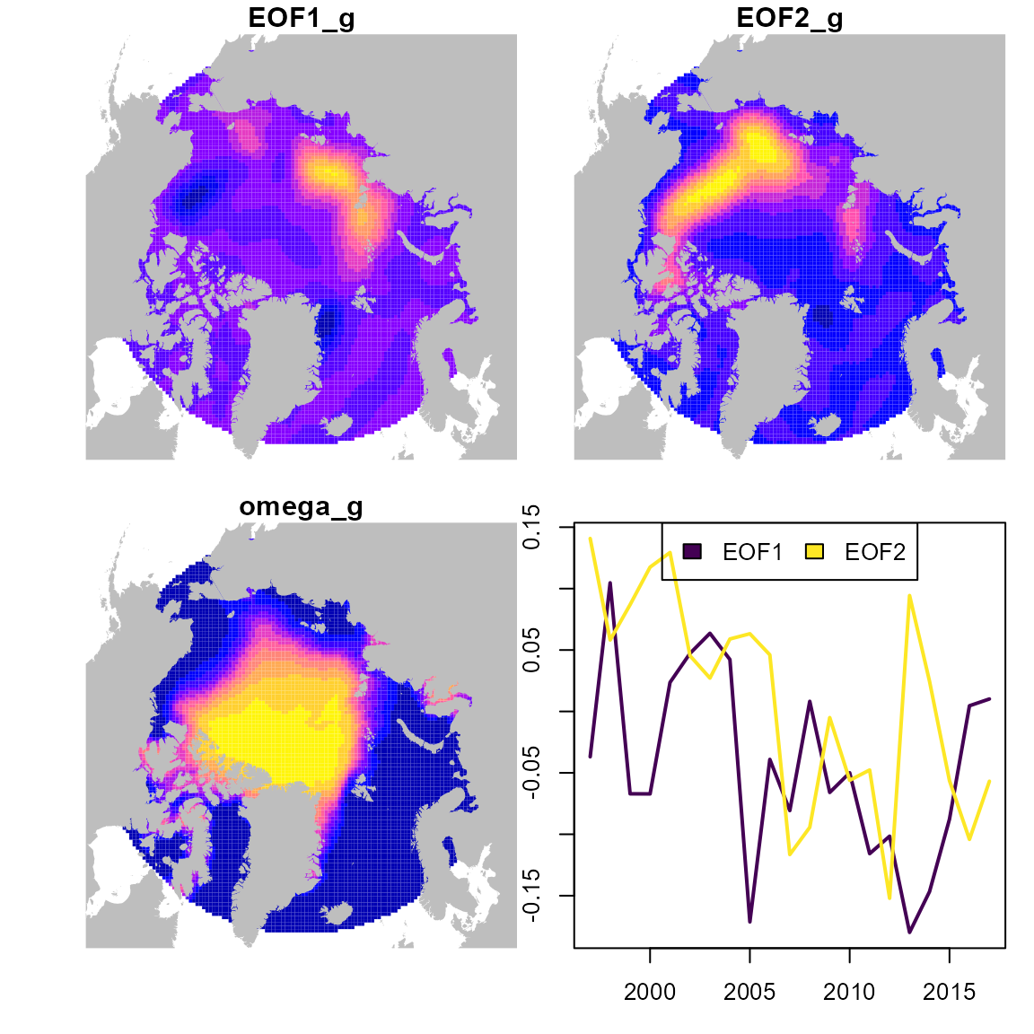

Runtime for this vignette: 3.78 mins

Works cited

Thorson, James T., Lorenzo Ciannelli, and Michael A. Litzow. 2020. “Defining Indices of Ecosystem Variability Using Biological Samples of Fish Communities: A Generalization of Empirical Orthogonal Functions.” Progress in Oceanography 181 (February): 102244. https://doi.org/10.1016/j.pocean.2019.102244.

James T. Thorson

Empirical Orthogonal Function (EOF) analysis

Works cited