Simultaneous autoregressive process

library(tinyVAST)
library(igraph)
library(rnaturalearth)
library(sf)
options("tinyVAST.verbose" = FALSE)

tinyVAST is an R package for fitting vector autoregressive spatio-temporal (VAST) models using a minimal and user-friendly interface. We here show how it can fit a multivariate second-order autoregressive (AR2) model including spatial correlations using a simultaneous autoregressive (SAR) process specified using igraph.

Load and format data

To do so, we first load salmong returns, and remove 0s to allow comparison between Tweedie and lognormal distributions.

data( salmon_returns )

# Transform data
salmon_returns$Biomass_nozeros = ifelse( salmon_returns$Biomass==0,
                                         NA, salmon_returns$Biomass )
Data = na.omit(salmon_returns)

Analysis

Independent dynamics among populations

We first explore an AR2 process, with independent variation among regions. This model shows a substantial first-order autocorrelation for sockeye and chum, and substantial second-order autocorrelation for pink salmon. An AR(2) process is stationary if $\phi_1 + \phi_2 < 1$ and $\phi_2 - \phi_1 < 1$ , and this stationarity criterion suggests that each time-series is close to (but not quite) nonstationary.

# Define graph for SAR process
unconnected_graph = make_empty_graph( nlevels(Data$Region) )
V(unconnected_graph)$name = levels(Data$Region)
plot(unconnected_graph)


# Define SEM for AR2 process
dsem = "
  sockeye -> sockeye, -1, lag1_sockeye
  sockeye -> sockeye, -2, lag2_sockeye

  pink -> pink, -1, lag1_pink
  pink -> pink, -2, lag2_pink

  chum -> chum, -1, lag1_chum
  chum -> chum, -2, lag2_chum
"

# Fit tinyVAST model
mytiny0 = tinyVAST(
     formula = Biomass_nozeros ~ 0 + Species + Region,
     data = Data,
     spacetime_term = dsem,
     variable_column = "Species",
     time_column = "Year",
     space_column = "Region",
     distribution_column = "Species",
     family = list( "chum" = lognormal(),
                          "pink" = lognormal(),
                          "sockeye" = lognormal() ),
     spatial_domain = unconnected_graph,
     control = tinyVASTcontrol( profile="alpha_j" ) )

# Summarize output
Summary = summary(mytiny0, what="spacetime_term")
knitr::kable( Summary, digits=3)

heads	to	from	parameter	start	lag	Estimate	Std_Error	z_value	p_value
1	sockeye	sockeye	1	NA	-1	0.808	0.059	13.710	0.000
1	sockeye	sockeye	2	NA	-2	0.195	0.059	3.307	0.001
1	pink	pink	3	NA	-1	0.050	0.019	2.640	0.008
1	pink	pink	4	NA	-2	0.882	0.022	39.933	0.000
1	chum	chum	5	NA	-1	0.675	0.103	6.582	0.000
1	chum	chum	6	NA	-2	0.292	0.100	2.939	0.003
2	pink	pink	7	NA	0	0.648	0.039	16.766	0.000
2	chum	chum	8	NA	0	0.294	0.035	8.349	0.000
2	sockeye	sockeye	9	NA	0	0.421	0.036	11.622	0.000

Spatially correlated dynamics among populations

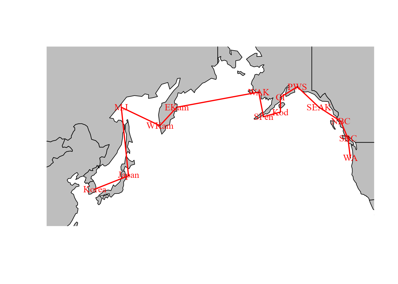
We also explore an SAR process for adjacency among regions

# Define graph for SAR process
adjacency_graph = make_graph( ~ Korea - Japan - M.I - WKam - EKam -
                                WAK - SPen - Kod - CI - PWS -
                                SEAK - NBC - SBC - WA )

We can plot this adjacency on a map to emphasize that it is a simple way to encode information about spatial proximity:

#maps = ne_countries( country = c("united states of america","russia","canada","south korea","north korea","japan") )
maps = ne_countries( continent = c("north america","asia","europe") )
maps = st_combine( maps )
maps = st_transform( maps, crs=st_crs(3832) )
#maps = st_crop( maps, xmin = -5*1e5, xmax = 12*1e5,
#                      ymin = 0 * 1e6, ymax=10 * 1e6 )

# Format inputs
loc_xy = cbind(
  x = c(129,143,140,156,163,-163,-161,-154,-154,-147,-138,-129,-126,-125),
  y = c(36,40,57,53,57,60,55,56,59,61,57,54,50,45)
)
loc_xy = sf_project( loc_xy, from=st_crs(4326), to=st_crs(3832) )

# Plot
xlim = c(-4,10) * 1e6
ylim = c(3,10) * 1e6
plot( maps, 
      xlim = xlim,
      ylim = ylim,
      col = "grey",
      asp = FALSE,
      add = FALSE )
plot( adjacency_graph, 
      layout = loc_xy,
      add = TRUE, 
      rescale = FALSE,
      vertex.label.color = "red",
      xlim = xlim, 
      ylim = ylim, 
      edge.width = 2,
      edge.color = "red" )

We can then pass this adjacency graph to tinyVAST during fitting:

# Fit tinyVAST model
mytiny = tinyVAST(
     formula = Biomass_nozeros ~ 0 + Species + Region,
     data = Data,
     spacetime_term = dsem,
     variable_column = "Species",
     time_column = "Year",
     space_column = "Region",
     distribution_column = "Species",
     family = list( "chum" = lognormal(),
                          "pink" = lognormal(),
                          "sockeye" = lognormal() ),
     spatial_domain = adjacency_graph,
     control = tinyVASTcontrol( profile="alpha_j" ) )

# Summarize output
Summary = summary(mytiny, what="spacetime_term")
knitr::kable( Summary, digits=3)

heads	to	from	parameter	start	lag	Estimate	Std_Error	z_value	p_value
1	sockeye	sockeye	1	NA	-1	1.505	0.081	18.529	0.000
1	sockeye	sockeye	2	NA	-2	-0.502	0.082	-6.113	0.000
1	pink	pink	3	NA	-1	0.010	0.009	1.093	0.274
1	pink	pink	4	NA	-2	0.978	0.010	100.558	0.000
1	chum	chum	5	NA	-1	1.685	0.113	14.978	0.000
1	chum	chum	6	NA	-2	-0.688	0.113	-6.108	0.000
2	pink	pink	7	NA	0	0.575	0.041	14.158	0.000
2	chum	chum	8	NA	0	0.077	0.023	3.421	0.001
2	sockeye	sockeye	9	NA	0	0.232	0.029	7.977	0.000

Model selection and visualization

We can use AIC to compare these two models. This comparison suggests that spatial adjancency is not a parsimonious way to describe correlations among time-series.

# AIC for unconnected time-series
AIC(mytiny0)
#> [1] 49086.47
# AIC for SAR spatial variation
AIC(mytiny)
#> [1] 49755.91

Finally, we can plot observations and predictions for the selected model

# Compile long-form dataframe of observations and predictions
Resid = rbind( cbind(Data[,c('Species','Year','Region','Biomass_nozeros')], "Which"="Obs"),
               cbind(Data[,c('Species','Year','Region')], "Biomass_nozeros"=predict(mytiny0,Data), "Which"="Pred") )

# plot using ggplot
library(ggplot2)
ggplot( data=Resid, aes(x=Year, y=Biomass_nozeros, col=Which) ) + # , group=yhat.id
  geom_line() +
  facet_grid( rows=vars(Region), cols=vars(Species), scales="free" ) +
  scale_y_continuous(trans='log')  #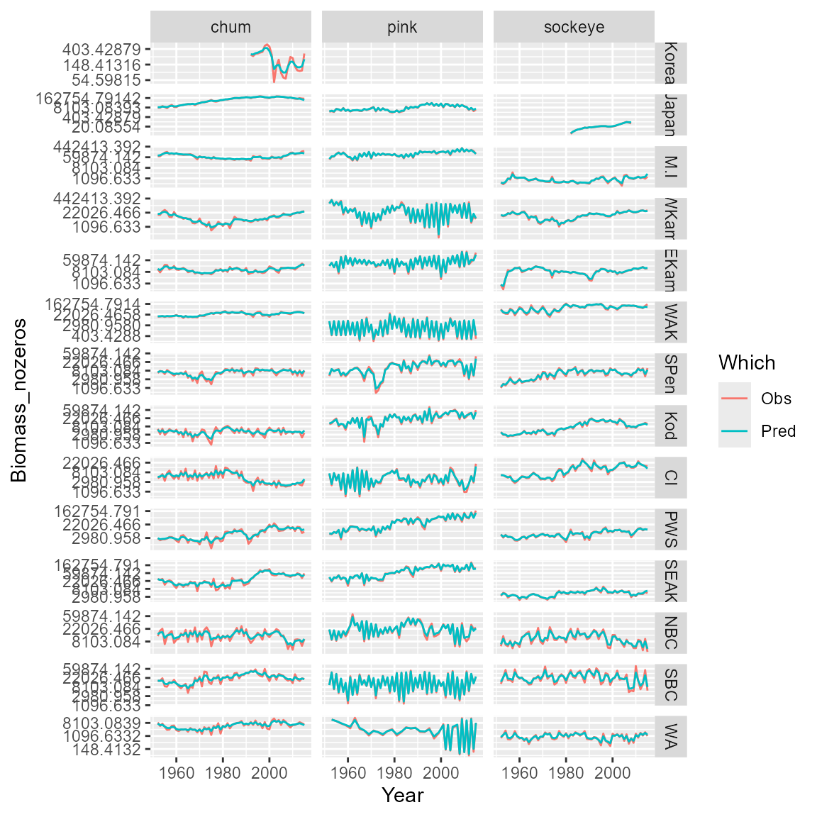

Runtime for this vignette: 8.76 secs

James T. Thorson

Load and format data

Analysis

Independent dynamics among populations

Spatially correlated dynamics among populations

Model selection and visualization

Works cited