Age composition expansion
James T. Thorson
Source:vignettes/web_only/age_composition_expansion.Rmd
age_composition_expansion.RmdtinyVAST is an R package for fitting vector autoregressive spatio-temporal (VAST) models. We here explore the capacity to use area-expansion to calculate proportion-at-age using spatially unbalanced sampling data (Thorson and Haltuch 2018).
Expanding age-composition data
To start, we load sampling data that has undergone first-stage expansion. This arises when each primary sampling unit includes secondary subsampling of ages, and the subsampled proportion-at-age in each primary unit has been expanded to the total abundance in that primary sample:
data( bering_sea_pollock_ages )

# subset to Years 2017-2023 (to speed up the example)
Data = subset( bering_sea_pollock_ages, Year >= 2017 )

# Add Year-_Age interaction
Data$Age = factor( paste0("Age_",Data$Age) )
Data$Year_Age = interaction( Data$Year, Data$Age )

# Project data to UTM
Data = st_as_sf(
  Data,
  coords = c('Lon','Lat'),
  crs = st_crs(4326)
)
Data = st_transform(
  Data,
  crs = st_crs("+proj=utm +zone=2 +units=km")
)

# Add UTM coordinates as columns X & Y
Data = cbind( st_drop_geometry(Data), st_coordinates(Data) )

# Make spatial domain
mesh = fm_mesh_2d(
  loc = Data[,c("X","Y")],
  cutoff = 50
)
Model specification
Next, we construct the various inputs to tinyVAST. We specify a separate variance for spatial variation by age, separate variance for spatio-temporal variation by age, and a shared magnitude of AR1 correlations over time. In other examples, the analyst might want to specify some of the spatial and spatio-temporal variance terms as having a value that is shared among ages, to ensure these variances are estimable:
# adds different variances for each age
sem = ""

# Constant AR1 spatio-temporal term across ages
# and adds different variances for each age
dsem = "
  Age_1 -> Age_1, 1, lag1
  Age_2 -> Age_2, 1, lag1
  Age_3 -> Age_3, 1, lag1
  Age_4 -> Age_4, 1, lag1
  Age_5 -> Age_5, 1, lag1
  Age_6 -> Age_6, 1, lag1
  Age_7 -> Age_7, 1, lag1
  Age_8 -> Age_8, 1, lag1
  Age_9 -> Age_9, 1, lag1
  Age_10 -> Age_10, 1, lag1
  Age_11 -> Age_11, 1, lag1
  Age_12 -> Age_12, 1, lag1
  Age_13 -> Age_13, 1, lag1
  Age_14 -> Age_14, 1, lag1
  Age_15 -> Age_15, 1, lag1
"

# Separate intercept for each Year-Age combination
Formula = Abundance_per_hectare ~ 0 + Year_Age

#
control = tinyVASTcontrol( getsd = FALSE,
                           profile = c("alpha_j"),
                           trace = 0 )
Fitting the model
We the fit the model with a log-linked Tweedie distribution and a single linear predictor:
# Define separate tweedie family for each age
Family = list(
  Age_1 = tweedie(),
  Age_2 = tweedie(),
  Age_3 = tweedie(),
  Age_4 = tweedie(),
  Age_5 = tweedie(),
  Age_6 = tweedie(),
  Age_7 = tweedie(),
  Age_8 = tweedie(),
  Age_9 = tweedie(),
  Age_10 = tweedie(),
  Age_11 = tweedie(),
  Age_12 = tweedie(),
  Age_13 = tweedie(),
  Age_14 = tweedie(),
  Age_15 = tweedie()
)

# Fit model
myfit = tinyVAST(
  data = Data,
  formula = Formula,
  space_term = sem,
  spacetime_term = dsem,
  family = Family,
  space_column = c("X", "Y"),
  variable_column = "Age",
  time_column = "Year",
  distribution_column = "Age",
  spatial_domain = mesh,
  control = control
)
Area expansion and proportions
After the model is fitted, we then apply area-expansion to predict abundance-at-age, and convert that to a proportion. Below, we forgo epsilon bias-correction (Thorson and Kristensen 2016), but we strongly recommend it for real-world applications to avoid proportion estimates being biased low for ages with fewer samples (and therefore higher standard errors):
# Get shapefile for survey extent
data( bering_sea )

# Make extrapolation grid based on shapefile
bering_sea = st_transform( bering_sea,
                           st_crs("+proj=utm +zone=2 +units=km") )
grid = st_make_grid( bering_sea, n=c(50,50) )
grid = st_intersection( grid, bering_sea )
grid = st_make_valid( grid )
loc_gz = st_coordinates(st_centroid( grid ))

# Get area for extrapolation grid
library(units)
areas = set_units(st_area(grid), "hectares") #  / 100^2 # Hectares

# Get abundance
N_jz = expand.grid( Age=myfit$internal$variables, Year=sort(unique(Data$Year)) )
N_jz = cbind( N_jz, "Biomass"=NA, "SE"=NA )
for( j in seq_len(nrow(N_jz)) ){
  if( N_jz[j,'Age']==1 ){
    message( "Integrating ", N_jz[j,'Year'], " ", N_jz[j,'Age'], ": ", Sys.time() )
  }
  if( is.na(N_jz[j,'Biomass']) ){
    newdata = data.frame( loc_gz, Year=N_jz[j,'Year'], Age=N_jz[j,'Age'])
      newdata$Year_Age = paste( newdata$Year, newdata$Age, sep="." )
    # Area-expansion
    index1 = integrate_output( myfit,
                    area = areas,
                    newdata = newdata,
                    apply.epsilon = FALSE,
                    bias.correct = FALSE,
                    intern = FALSE,
                    getsd = FALSE )
    #N_jz[j,'Biomass'] = index1[3] / 1e9
    N_jz[j,'Biomass'] = index1[1] / 1e9
  }
}
N_ct = array(
  N_jz$Biomass,
  dim = c(length(myfit$internal$variables),length(unique(Data$Year))),
  dimnames = list(myfit$internal$variables,sort(unique(Data$Year)))
)
N_ct = sweep( N_ct, MARGIN = 1, FUN = "/", STATS = colSums(N_ct) )
#> Warning in sweep(N_ct, MARGIN = 1, FUN = "/", STATS = colSums(N_ct)): STATS
#> does not recycle exactly across MARGIN
Comparison with VAST
Finally, we can compare these estimates with those from package VAST (Thorson and Barnett 2017). Estimates differ somewhat because VAST used a delta-gamma distribution with spatio-temporal variation in two linear predictors, used a different mesh, and we also skipped epsilon bias-correction for tinyVAST to have a faster-running vignette.
# Load VAST results for same data
data(bering_sea_pollock_vast)
myvast = bering_sea_pollock_vast
rownames(myvast) = 1:15

# Reformat tinyVAST output with same dimnames
mytiny = N_ct
rownames(mytiny) = 1:15

# Combine in long-form data frame (expected by ggplot)
longvast = cbind(
  expand.grid(dimnames(myvast)),
  p = as.numeric(myvast),
  method = "VAST" )
longtiny = cbind(
  expand.grid(dimnames(mytiny)),
  p = as.numeric(mytiny),
  method = "tinyVAST" )
long = rbind( longvast, longtiny )

# Plot with facet by age
library(ggplot2)
ggplot( data=long, aes(x=Var2, y=p, col=method) ) +
  facet_grid( rows=vars(Var1), scales="free" ) +
  geom_point( ) +
  scale_y_log10()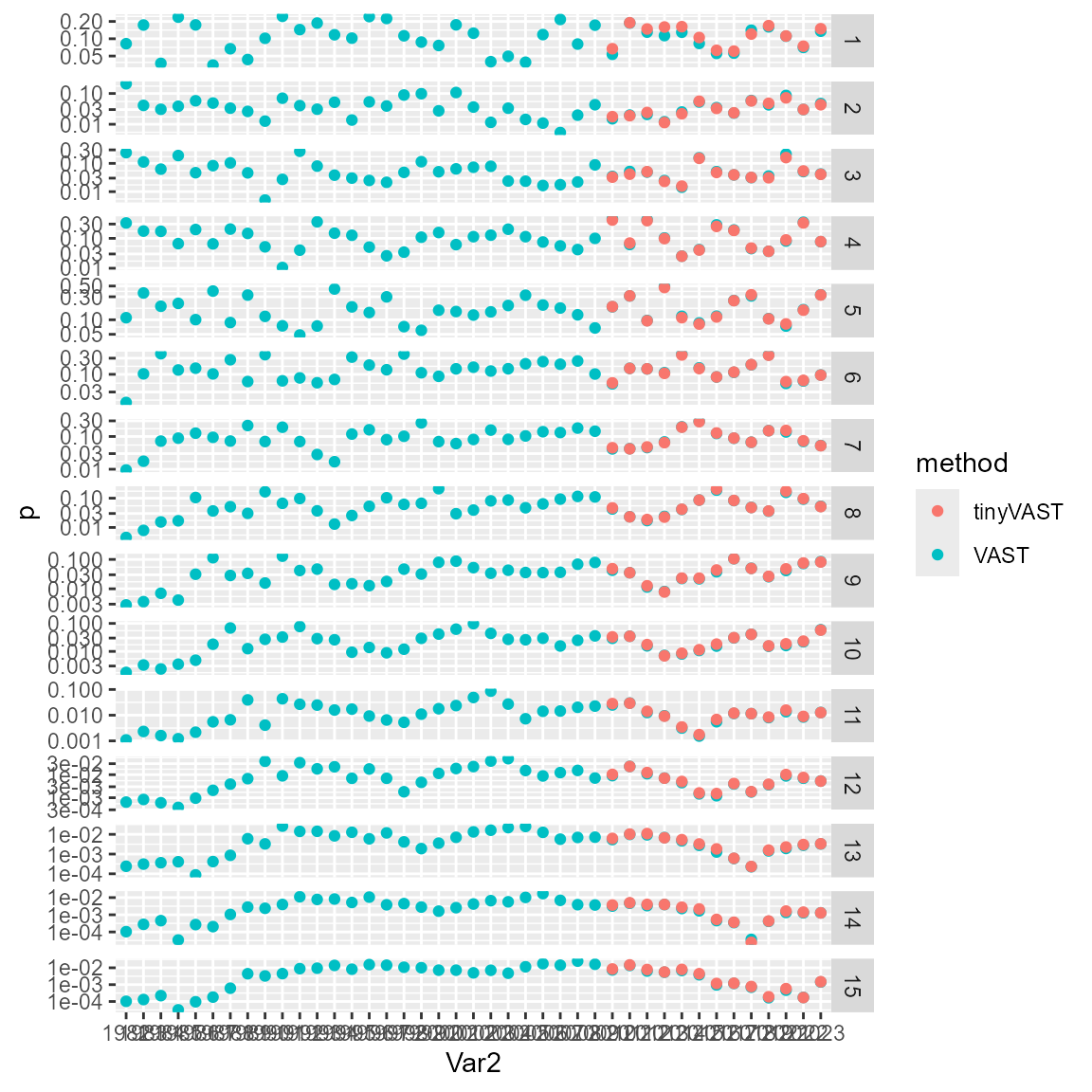
Runtime for this vignette: 15.82 mins